Geometric Anisotropy

A semi-variogram $/gamma(h_u, h_v, h_w)$ or a covariance $C(h_u, h_v, h_w)$ has a geometric anisotropy when the anisotropy can be reduced to isotropy by a mere linear transformation of the coordinates:

with

or, in matrix form,

where $A = a_{ij}$ represents the matrix of transformation of the coordinates, and ${/boma h}$ and ${/boma h}'$ are column-vectors of the coordinates.

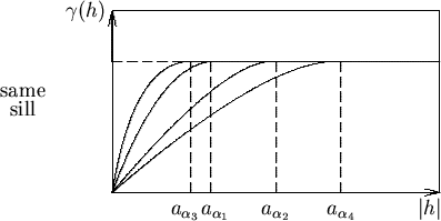
An example is given in Figure 4.6, which shows four semi-variograms for four horizontal directions $/alpha_1, /alpha_2, /alpha_3, /alpha_4$. Spherical models with identical sills and ranges of $a_{/alpha_1}, a_{/alpha_2}, a_{/alpha_3}, a_{/alpha_4}$ have been fitted to these semi-variograms. The directional graph of the ranges, i.e., the variation of the ranges $a_{/alpha_i}$ as a function of the direction $/alpha_i$, is also shown in Figure 4.5. There are three possible cases.

Figure 4.5: Ranges in Case of Anisotropy.

Figure 4.6: Geometric Anisotropy.

(i)

The graph can be approximated to a circle of radius $a$, i.e., $a_{/alpha_i} /cong a$, for all horizontal directions $/alpha_i$ and the phenomenon can thus be considered as isotropic and characterized by a spherical model of range $a$.

(ii)

The graph can be approximated by an ellipse, i.e., by a shape which is a linear transform of a circle. By applying this linear transformation to the coordinates of vector $/boma h$, the isotropic case is produced (circular graph). The phenomenon is a geometric anisotropy.

(iii)

The graph cannot be fitted to a second-degree curve and the second type of anisotropy must be considered, i.e., zonal anisotropy in certain directions, $/alpha_4$, for example, on Figure 4.5.

If, instead of transition structures of range $a_{/alpha_i}$ as in Figure 4.5, the directional semi-variograms are of the linear type, $/gamma_{/alpha_i}(h_i) = /omega_{/alpha_i} h_i$, then the directional graphs of the inverses of the slopes at the origin $/omega_{/alpha_i}$ will be considered. A hypothesis of isotropy, geometric anisotropy or zonal anisotropy will then be adopted according to whether or not this directional graph can be fitted to a circle or an ellipse.