


Next: Remark 1
Up: Anisotropies
Previous: Geometric Anisotropy
Contents
Consider a geometric anisotropy in two dimensions (e.g., the horizontal
space). The directional graph of the ranges  is elliptical.
Let
is elliptical.
Let  be the initial rectangular coordinates of a point,
  the angle
made by the major axis of the ellipse with the coordinate axis
the angle
made by the major axis of the ellipse with the coordinate axis  , and
, and
 the ratio of anisotropy of the ellipse. The three following steps will
transform this ellipse into a circle and, thus, reduce the anisotropy to
isotropy.
the ratio of anisotropy of the ellipse. The three following steps will
transform this ellipse into a circle and, thus, reduce the anisotropy to
isotropy.
- (i)
- The first step is to rotate the coordinate axes by the angle so that
they become parallel to the main axes of the ellipse. The new
coordinates
 resulting from the rotation can be written in
matrix notation as
resulting from the rotation can be written in
matrix notation as
where  is the matrix of rotation through the angle .
- (ii)
- The second step is to transform the ellipse into a circle with a radius
equal to the major range of the ellipse. This is achieved by multiplying
the coordinate
 by the ratio of anisotropy . The new
coordinates
by the ratio of anisotropy . The new
coordinates  are then deduced from the coordinates
by the matrix expression
are then deduced from the coordinates
by the matrix expression
- (iii)
- The initial orientation of the coordinate system is then restored by
rotation through the angle
 , and the final transformed coordinates
 are given by
The final transformed coordinates can then be derived from
the initial coordinates by the transformation matrix  which is the product of the three matrices
 , i.e.,
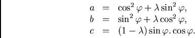
with
and
If  is any vector in the two-dimensional space with initial coordinates
 , then, to obtain the value of the anisotropic
semi-variogram
, then, to obtain the value of the anisotropic
semi-variogram
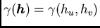 , we first calculate the transformed
coordinates
, we first calculate the transformed
coordinates  from
from
and then we substitute these coordinates in the isotropic model
 , which has a range equal to the major range of the directional
ellipse, i.e.,
, which has a range equal to the major range of the directional
ellipse, i.e.,
Next: Remark 1
Up: Anisotropies
Previous: Geometric Anisotropy
Contents
Rudolf Dutter
2003-03-13
![/begin{displaymath}/left[ /begin{array}{l}y_1// y_2/end{array}/right] = R_/varph...
.../varphi// -/sin /varphi & /cos /varphi
/end{array}/right]/ / , /end{displaymath}](img498.png)
![/begin{displaymath}/left[ /begin{array}{l}y_1'// y_2'/end{array}/right] = /lambd...
...[
/begin{array}{cc}1 & 0// 0 & /lambda
/end{array}/right]/ / . /end{displaymath}](img502.png)
![/begin{displaymath}/left[ /begin{array}{l}x_u'// x_v'/end{array}/right] = R_{-/varphi}
/left[ /begin{array}{l}y_1'// y_2'/end{array}/right]/end{displaymath}](img505.png)
![/begin{displaymath}/left[ /begin{array}{l}x_u'// x_v'/end{array}/right] = R_{-/v...
...}/right] =
A/left[ /begin{array}{l}x_u// x_v/end{array}/right]/end{displaymath}](img508.png)
![/begin{displaymath}A = /left[
/begin{array}{cc}a & c// c & b
/end{array}/right]/ / . /end{displaymath}](img509.png)
![/begin{displaymath}/left[ /begin{array}{l}h_u'// h_v'/end{array}/right] = A
/left[ /begin{array}{l}h_u// h_v/end{array}/right]/end{displaymath}](img514.png)