Case Study: 3-dimensional Kriging with an Older Computer Program

In this section we discuss a complex case study to show how it would typically be performed using a large, classical computer program (Maréchal, 1980[14]). We don't put much intension on theoretical and computational details rather than on the practical use of the computer. In case of many data values in the 3-dimensional space, as in mining of a saline, the organization of the data and the processing already is problematic. In order to keep the computing time for the analysis within feasible limits, the special computer configurations have to be considered. For the following study the data set was provided together with the program package GEOSLIB. The installation was done on a UNIVAC 1100/81 and the main difficulties in the computer center (TU Graz) at that time were the data access and handling of this ``large'' set (Pichler, 1982[17]).

The problem is the investigation of an ore deposit with 79 drill holes which are placed at a regular grid of

meter. Identification numbers of the holes together with their

-coordinates are reproduced in Figure 6.4.

**Table 6.1:** Original- and Regularized Data.
17 440.004870.00 36.00
440.004870.00	35.00	3.200	5.824
440.004870.00	34.00	3.200	5.824
440.004870.00	33.00	8.000	7.920
440.004870.00	32.00	8.100	7.047
440.004870.00	31.00	25.500	6.375
440.004870.00	30.00	10.500	4.410
440.004870.00	29.00	18.000	4.680
440.004870.00	28.00	17.000	2.720
440.004870.00	27.00	16.700	10.855
440.004870.00	26.00	8.200	9.922
440.004870.00	25.00	30.200	7.248
440.004870.00	24.00	33.600	6.384
440.004870.00	23.00	36.700	7.707
440.004870.00	22.00	37.200	8.556
440.004870.00	21.00	38.500	7.700
440.004870.00	20.00	37.500	7.125
440.004870.00	19.00	39.200	7.840
17 440.004880.00 36.00
440.004880.00	35.00	3.900	2.730
440.004880.00	34.00	3.900	2.730
440.004880.00	33.00	4.000	3.920
440.004880.00	32.00	21.900	6.570
440.004880.00	31.00	8.600	5.246
440.004880.00	30.00	10.700	8.132
440.004880.00	29.00	10.000	6.800
440.004880.00	28.00	9.700	6.596
440.004880.00	27.00	25.800	9.546
440.004880.00	26.00	26.200	10.480
440.004880.00	25.00	29.400	10.290
440.004880.00	24.00	27.500	8.525
440.004880.00	23.00	23.500	7.285
440.004880.00	22.00	30.500	8.845
440.004880.00	21.00	22.200	6.438
440.004880.00	20.00	27.400	7.124
440.004880.00	19.00	30.600	7.956
17 440.004890.00 36.00
440.004890.00	35.00	6.000	5.640
440.004890.00	34.00	4.500	4.050
440.004890.00	33.00	8.300	9.296
440.004890.00	32.00	10.500	8.190
440.004890.00	31.00	12.300	6.273
440.004890.00	30.00	13.200	4.620
440.004890.00	29.00	10.300	4.635
440.004890.00	28.00	9.700	5.044
440.004890.00	27.00	23.300	7.223
440.004890.00	26.00	21.300	5.538
440.004890.00	25.00	17.400	5.742
440.004890.00	24.00	13.300	5.054
440.004890.00	23.00	13.300	4.256
440.004890.00	22.00	26.200	6.812
440.004890.00	21.00	26.300	7.627
440.004890.00	20.00	24.300	6.318
440.004890.00	19.00	22.900	6.412
18 430.004870.00 36.00
Original Data

8 440.004870.00 36.00
440.004870.00	34.00	3.200	5.824
440.004870.00	32.00	8.050	7.484
440.004870.00	30.00	18.000	5.392
440.004870.00	28.00	17.500	3.700
440.004870.00	26.00	12.450	10.388
440.004870.00	24.00	31.900	6.816
440.004870.00	22.00	36.950	8.132
440.004870.00	20.00	38.000	7.412
8 440.004880.00 36.00
440.004880.00	34.00	3.900	2.730
440.004880.00	32.00	12.950	5.245
440.004880.00	30.00	9.650	6.689
440.004880.00	28.00	9.850	6.698
440.004880.00	26.00	26.000	10.013
440.004880.00	24.00	28.450	9.407
440.004880.00	22.00	27.000	8.065
440.004880.00	20.00	24.800	6.781
8 440.004890.00 36.00
440.004890.00	34.00	5.250	4.845
440.004890.00	32.00	9.400	8.743
440.004890.00	30.00	12.750	5.447
440.004890.00	28.00	10.000	4.4840
440.004890.00	26.00	22.300	6.380
440.004890.00	24.00	15.350	5.398
440.004890.00	22.00	19.750	5.534
440.004890.00	20.00	25.300	6.972
8 430.004870.00 36.00
430.004870.00	34.00	32.000	11.466
430.004870.00	32.00	34.550	7.795
430.004870.00	30.00	35.750	8.197
430.004870.00	28.00	24.750	19.701
430.004870.00	26.00	18.650	35.807
430.004870.00	24.00	23.800	19.729
430.004870.00	22.00	26.750	11.844
430.004870.00	20.00	32.550	7.486
8 430.004880.00 36.00
430.004880.00	34.00	32.800	6.560
430.004880.00	32.00	32.250	5.160
430.004880.00	30.00	28.600	4.146
430.004880.00	28.00	23.100	4.227
430.004880.00	26.00	6.300	13.139
430.004880.00	24.00	2.750	12.537
430.004880.00	22.00	15.650	23.329
430.004880.00	20.00	9.900	14.222
8 430.004890.00 36.00
430.004890.00	34.00	35.900	8.616
430.004890.00	32.00	36.950	6.477
430.004890.00	30.00	29.450	4.575
430.004890.00	28.00	24.700	3.670
430.004890.00	26.00	39.750	6.757
430.004890.00	24.00	42.050	8.500
430.004890.00	22.00	40.850	7.340
430.004890.00	20.00	40.600	41.320
8 430.004900.00 36.00
Regularized Data

In each heading of a drill hole the number of core samples and the identification, say the

- and

-coordinates ( $x_{u}$ and $x_{v}$ ) and the starting level of the measurements are given. After the heading a row for each measurement is used: $x_{u}, x_{v}$ and $x_{w}$ as well the values of both variables called 1st Var. and 2nd Var..

The goal of the study is the computation of the estimated mean values as well as the estimation variances of both variables in equally sized blocks of

meter. The different steps of this performance are shown in the flow diagram of Figure 6.5.

In order the make the data feasible, they need to be regularized. For our case the program CLAS2 produces data in each drill hole for cores of length 2 meter. The result is stored in a file named WORK.REGUDAT. The first records are also listed in Table 6.1.

**Figure 6.5:** Flow Diagram of an Example of Kriging.
$/begin{figure}/centerline{/psfig{figure=fig6_5.eps,height=180mm}}/end{figure}$

The first branch of the diagram (Figure 6.5) considers the data non structured, i.e. independently generated, and computes simple statistics. HIST draws histograms, MATC scattergrams and CORL computes correlations. The so produced histogram of the first variable is presented in the output of Figure 6.6. The empirical distribution appears to be left skewed, which is rather rare in geostatistical applications. 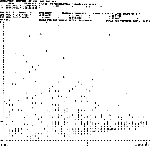The opposite is the case with variable ``2nd Var.''. The histogram is not reproduced, however, it may be seen from the scattergram in Figure 6.7 (in the marginal distribution). There the correlation coefficient of -.30 is also displayed.

**Figure 6.6:** Histogram of *``1st Var.''*.
$/begin{figure}/centerline{/psfig{figure=fig6_6.ps,height=140mm}}/end{figure}$

**Figure 6.7:** Scattergram of *``1st Var.''* and *``2nd Var.''*.
$/begin{figure}/centerline{/psfig{figure=fig6_7.ps,height=140mm}}/end{figure}$

In the second branch the proper structural analysis is performed. Different variograms are computed and graphically presented. In the vertical direction we compute only one variogram which is done by the program GAM1C. (``C'' also stands for

ovariogram). The program also provides a graphical output on the printer (see e.g. Figure 6.8). It is very advantageous if one has at hand a graphical screen and the presented data may be fitted interactively (by hand). Figure 6.8 shows a copy of such a graphic with the First Variable. The fitted, twice nested, spherical variogram with $C_{1}=36, a_{1}=5,$ $C_{2}=64$ and $a_{2}=17$ is drawn. There is a similar situation with the second variable. The graphic with the fitted variogram is shown in Figure 6.9.

**Figure 6.8:** Variogram of the First Variable in Vertical Direction.
$/begin{figure}/centerline{/psfig{figure=fig6_8.ps,width=11.5cm}}/end{figure}$

**Figure 6.9:** Variogram of the Second Variable in Vertical Direction.
$/begin{figure}/centerline{/psfig{figure=fig6_9.ps,width=11.5cm}}/end{figure}$

The horizontal plane (in case that this is a distinct direction) opens much more possibilities for computing variograms. E.g. in each plane of the sample points (core samples) a variogram may be calculated, and such ones in different directions in the plane. This is also strongly suggested for understanding the structure of the region. The program GAM2V offers the possibility of the computation in different directions. We only present the final result for the two variables in Figure 6.10 and Figure 6.11. Again twice nested, spherical variograms were used, and the First Variable seems to be isotropic. The Second Variable in the second variogram in horizontal direction seems to show a range which is half the size the range in vertical direction. This is expressed in the anisotropy factors (abbreviated ANIS).

**Figure 6.10:** Variogram of the First Variable in Horizontal Direction.
$/begin{figure}/centerline{/psfig{figure=fig6_10.ps,width=11.5cm}}/end{figure}$

**Figure 6.11:** Variogram of the Second Variable in Horizontal Direction.
$/begin{figure}/centerline{/psfig{figure=fig6_11.ps,width=11.5cm}}/end{figure}$

The found parameters of the fitted variogram models must be entered in a data file to be reread in the later kriging procedure. In our case using the computer system UNIVAC the file is called WORK.PARADAT (see Figure 6.5), in which also other ``kriging parameters'' must be specified. E.g. we list the contents of this file in Table 6.2 where also the numbers of blocks of the neighborhood are specified. Besides the found geometric anisotropies, we can also take advantage from isotropy (e.g. within the horizontal planes). With this isotropy assumption the sample points with constant distance in such a plane get the same weight. This is specified in the rows labelled with ``Identification of blocks/weights'' in Table 6.2. The small drawing beside should help identify the neighboring blocks of block nr. 14, and we see that the blocks 5 and 23 get the same weight, as well as 11, 13, 15 and 17, etc.

Figure 6.12: Table of the Drill Hole Numbers, generated by VUE.

        VARIABLE :HOLE            XOY CROSS-SECTION NUMBER :       1
    LOCATION OF THE     :  KZ=       1    I1=       1  I2=       8  
        CROSS-SECTION      -----------    J1=       1  J2=      11  
       1    2    3    4    5    6    7    8 
    *----*----*----*----*----*----*----*----*   
  1 ! 79 ! 68 ! 57 ! 46 ! 35 ! 24 !    !    !   
    *----*----*----*----*----*----*----*----*   
  2 ! 78 ! 67 ! 56 ! 45 ! 34 ! 23 ! 13 !    !   
    *----*----*----*----*----*----*----*----*   
  3 ! 77 ! 66 ! 55 ! 44 ! 33 ! 22 ! 12 !    !   
    *----*----*----*----*----*----*----*----*   
  4 ! 76 ! 65 ! 54 ! 43 ! 32 ! 21 ! 11 !    !   
    *----*----*----*----*----*----*----*----*   
  5 ! 75 ! 64 ! 53 ! 42 ! 31 ! 20 ! 10 !    !   
    *----*----*----*----*----*----*----*----*   
  6 ! 74 ! 63 ! 52 ! 41 ! 30 ! 19 !  9 !    !   
    *----*----*----*----*----*----*----*----*   
  7 ! 73 ! 62 ! 51 ! 40 ! 29 ! 18 !  8 !    !   
    *----*----*----*----*----*----*----*----*   
  8 ! 72 ! 61 ! 50 ! 39 ! 28 ! 17 !  7 !    !   
    *----*----*----*----*----*----*----*----*   
  9 ! 71 ! 60 ! 49 ! 38 ! 27 ! 16 !  6 !  3 !   
    *----*----*----*----*----*----*----*----*   
 10 ! 70 ! 59 ! 48 ! 37 ! 26 ! 15 !  5 !  2 !   
    *----*----*----*----*----*----*----*----*   
 11 ! 69 ! 58 ! 47 ! 36 ! 25 ! 14 !  4 !  1 !   
    O----*----*----*----*----*----*----*----*

The third branch shows that the data are reorganized by the program CLAS4, reordered in regular ``parallel epipedes'' and stored in file CLAS4.DAT for the (relatively) fast access for the kriging program.

The forth branch defines an envelope which comprises all blocks to be kriged. These indicators will be stored in the file IEXP.DAT. The contents of these two files may be displayed by the auxiliary program VUE.

Figure 6.13: Table of the Values of the 2 $^{nd}$ Variable in the 8 $^{nd}$ Level, generated by VUE.

        VARIABLE :2ND VAR         XOY CROSS-SECTION NUMBER :       8
    LOCATION OF THE     :  KZ=       8    I1=       1  I2=       8  
        CROSS-SECTION      -----------    J1=       1  J2=      11  
       1      2      3      4      5      6      7      8   
    *------*------*------*------*------*------*------*------*   
  1 ! 31.6 !  6.8 !  9.0 ! 16.4 !  8.1 !  6.0 !      !      !   
    *------*------*------*------*------*------*------*------*   
  2 !  8.4 !  6.5 !  4.4 !  3.1 !  7.2 !  7.3 !  5.8 !      !   
    *------*------*------*------*------*------*------*------*   
  3 !  5.2 ! 15.5 !  9.1 !  5.4 !  8.4 !  8.3 !  8.0 !      !   
    *------*------*------*------*------*------*------*------*   
  4 !  6.5 !  4.0 !  6.5 !  6.0 !  5.3 !  9.1 !  8.1 !      !   
    *------*------*------*------*------*------*------*------*   
  5 !  7.3 ! 44.8 !  9.5 !  6.9 !  5.6 !  7.5 !  8.5 !      !   
    *------*------*------*------*------*------*------*------*   
  6 ! 17.7 !  6.3 !  3.4 ! 13.7 !  5.3 !  6.8 !  5.7 !      !   
    *------*------*------*------*------*------*------*------*   
  7 !  6.5 !  7.3 !  5.7 !  7.0 !  6.5 !  7.4 !  7.3 !      !   
    *------*------*------*------*------*------*------*------*   
  8 !  7.3 !  5.3 !  4.7 !  6.5 ! 11.3 !  9.1 !  6.2 !      !   
    *------*------*------*------*------*------*------*------*   
  9 ! 13.9 !  7.8 !  7.8 !  4.1 !  5.2 !  7.3 ! 41.3 !  7.0 !   
    *------*------*------*------*------*------*------*------*   
 10 ! 17.8 ! 18.5 ! 33.2 !  8.6 !  5.1 !  9.3 ! 14.2 !  6.8 !   
    *------*------*------*------*------*------*------*------*   
 11 !  4.8 !  6.8 !  6.2 !  8.9 ! 15.2 ! 38.8 !  7.5 !  7.4 !   
    O------*------*------*------*------*------*------*------*

The essential parameters for the kriging, the summary of the weighting factors and the definition of the variogram models are printed at the beginning once more by the kriging program (see the output in Figure 6.14).

**Figure 6.14:** Printed Specifications by the Kriging Program.
$/begin{figure}/centerline{/psfig{figure=fig6_14.ps,height=140mm}}/end{figure}$

Now we perform the proper kriging, i.e. the computation of the averaged variograms and of the estimated averaged block values. A small excerpt of the produced listing is presented in the output of Figure 6.15. For the highest layer and a panel in the

-direction, the estimated averaged values and variances of the blocks as well as the computed values of

and $/lambda_{i}, /; i=1,/ldots 6$ are given. The complete output, however, is written on file KRIG.DAT, which may again be visualized by the program VUE. The output of Figure 6.16 e.g. shows a layer of estimated mean values and estimation variances of all blocks to be estimated.

**Figure 6.15:** Estimated Mean Values, Variances and Weight Factors.
$/begin{figure}/centerline{/psfig{figure=fig6_15.ps,height=140mm}}/end{figure}$

Figure 6.16: Kriging Estimates for Mean Values and Variances of both Variables.

    LOCATION OF THE     :  KZ=       1    I1=       1  I2=       8  
        CROSS-SECTION      -----------    J1=       1  J2=      11  
       1       2       3       4       5       6       7       8
    *-------*-------*-------*-------*-------*-------*-------*-------*   
  1 !  17.1 !  25.7 !  23.2 !  25.9 !  28.8 !  28.1 !  20.0 !   3.0 !   
    !  17.8 !  15.2 !  15.2 !  15.2 !  15.2 !  16.4 !  52.5 ! 116.7 !   
    !   5.9 !   6.2 !   7.8 !   8.2 !   6.8 !   5.3 !   5.3 !   5.2 !   
    !  10.6 !   8.8 !   8.8 !   8.8 !   8.8 !   9.6 !  19.8 !  45.2 !   
    *-------*-------*-------*-------*-------*-------*-------*-------*   
  2 !  26.4 !  29.4 !  23.9 !  29.7 !  34.1 !  30.4 !  12.4 !   4.0 !   
    !  15.2 !  13.6 !  13.6 !  13.6 !  13.6 !  13.7 !  16.2 !  70.2 !   
    !   9.7 !   8.2 !   6.8 !   7.9 !   7.2 !   5.5 !   5.6 !   5.2 !   
    !   8.8 !   7.7 !   7.7 !   7.7 !   7.7 !   7.9 !   9.6 !  26.1 !   
    *-------*-------*-------*-------*-------*-------*-------*-------*   
  3 !  21.7 !  27.8 !  19.7 !  27.4 !  33.5 !  31.5 !  12.1 !   5.4 !   
    !  15.2 !  13.6 !  13.6 !  13.6 !  13.6 !  13.6 !  14.7 !  59.0 !   
    !  18.6 !   8.4 !   6.6 !   6.9 !   6.6 !   5.9 !   5.5 !   5.1 !   
    !   8.8 !   7.7 !   7.7 !   7.7 !   7.7 !   7.7 !   8.8 !  20.1 !   
    *-------*-------*-------*-------*-------*-------*-------*-------*   
  4 !  20.0 !  27.9 !  29.3 !  24.3 !  32.7 !  30.3 !  14.3 !   9.7 !   
    !  15.2 !  13.6 !  13.6 !  13.6 !  13.6 !  13.6 !  14.7 !  59.0 !   
    !  12.6 !  10.4 !   6.2 !   5.2 !   6.6 !   6.7 !   6.5 !   4.6 !   
    !   8.8 !   7.7 !   7.7 !   7.7 !   7.7 !   7.7 !   8.8 !  20.1 !   
    *-------*-------*-------*-------*-------*-------*-------*-------*   
  5 !  17.4 !  22.9 !  24.2 !  26.5 !  27.2 !  28.4 !  17.4 !  12.2 !   
    !  15.2 !  13.6 !  13.6 !  13.6 !  13.6 !  13.6 !  14.7 !  59.0 !   
    !  13.5 !   8.6 !   6.7 !   5.6 !   6.4 !  10.4 !   6.1 !   4.0 !   
    !   8.8 !   7.7 !   7.7 !   7.7 !   7.7 !   7.7 !   8.8 !  20.1 !   
    *-------*-------*-------*-------*-------*-------*-------*-------*   
  6 !  21.5 !  23.4 !  18.4 !  22.9 !  24.2 !  27.6 !  19.1 !  20.3 !   
    !  15.2 !  13.6 !  13.6 !  13.6 !  13.6 !  13.6 !  14.7 !  59.0 !   
    !  11.6 !   9.8 !   7.6 !   9.1 !   9.1 !   9.0 !  10.1 !   4.5 !   
    !   8.8 !   7.7 !   7.7 !   7.7 !   7.7 !   7.7 !   8.8 !  20.1 !   
    *-------*-------*-------*-------*-------*-------*-------*-------*   
  7 !  20.0 !  28.6 !  26.5 !  26.7 !  23.2 !  26.0 !  30.5 !  27.9 !   
    !  15.2 !  13.6 !  13.6 !  13.6 !  13.6 !  13.6 !  14.7 !  59.0 !   
    !   9.7 !  10.0 !   9.1 !   7.8 !  10.5 !  16.7 !  10.2 !   5.6 !   
    !   8.8 !   7.7 !   7.7 !   7.7 !   7.7 !   7.7 !   8.8 !  20.1 !   
    *-------*-------*-------*-------*-------*-------*-------*-------*   
  8 !  26.6 !  27.6 !  27.2 !  20.7 !  24.9 !  31.2 !  32.8 !  26.4 !   
    !  15.2 !  13.6 !  13.6 !  13.6 !  13.6 !  13.6 !  14.4 !  47.9 !   
    !   7.2 !   7.1 !   9.8 !  10.4 !   9.8 !  10.2 !  10.9 !   6.9 !   
    !   8.8 !   7.7 !   7.7 !   7.7 !   7.7 !   7.7 !   8.3 !  16.9 !   
    *-------*-------*-------*-------*-------*-------*-------*-------*   
  9 !  27.5 !  26.2 !  28.8 !  28.2 !  23.7 !  32.1 !  31.2 !  15.1 !   
    !  15.2 !  13.6 !  13.6 !  13.6 !  13.6 !  13.6 !  13.7 !  16.2 !   
    !   9.9 !   8.1 !   7.4 !   6.9 !   7.4 !   9.6 !   7.9 !   6.1 !   
    !   8.8 !   7.7 !   7.7 !   7.7 !   7.7 !   7.7 !   7.9 !   9.6 !   
    *-------*-------*-------*-------*-------*-------*-------*-------*   
 10 !  20.3 !  29.5 !  28.4 !  26.7 !  20.2 !  20.6 !  27.1 !  12.7 !   
    !  15.2 !  13.6 !  13.6 !  13.6 !  13.6 !  13.6 !  13.6 !  14.7 !   
    !  13.2 !   9.1 !   7.2 !   6.0 !   7.5 !   9.1 !   8.3 !   5.9 !   
    !   8.8 !   7.7 !   7.7 !   7.7 !   7.7 !   7.7 !   7.7 !   8.8 !   
    *-------*-------*-------*-------*-------*-------*-------*-------*   
 11 !  22.0 !  28.4 !  27.5 !  27.8 !  21.1 !  19.8 !  25.5 !  12.3 !   
    !  17.2 !  14.7 !  14.7 !  14.7 !  14.7 !  14.7 !  14.7 !  16.6 !   
    !  10.1 !   8.9 !   6.3 !   6.7 !   9.4 !  11.2 !   9.4 !   6.5 !   
    !  10.6 !   8.8 !   8.8 !   8.8 !   8.8 !   8.8 !   8.8 !  10.5 !   
    O-------*-------*-------*-------*-------*-------*-------*-------*   
        VARIABLE :KRIGING         XOY CROSS-SECTION NUMBER :       2