The Lognormal Distribution

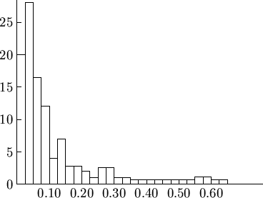
Applied work shows that values of ore samples do usually not follow the normal distribution, however, the logarithm of the values might much better be approximated by a normal distribution. This can be observed especially frequently in ore deposits with low grades, or when investigating geochemical data (trace elements). The distribution is right skewed (skewness is positive), and a typical histogram of samples from a gold mine is presented in Figure 2.9.

Figure 2.9: Histogram of Samples from a Gold Mine.

The density function $f$ is defined by

The transformed variable $Y /; = /; ln Z$ is normally distributed as $N(/mu,/beta^{2})$. After the transformation $y_{i}=ln /; z_{i}$ of the data, the parameters $/mu$ and $/beta$ may be estimated as in case of the normal distribution, namely as

Using the original data, $/hat{/mu}$ can also be found via the geometric mean:

or

An equivalent estimator of $e^/mu$ also is the median of the untransformed data.

Example 2.5: In the following two tables (Koch and Link, 1970-71[13]) we see frequencies of grades of samples of gold. One can immediately see the difficulties for the estimation of $/mu$.

Frequency Distribution of 1536 Gold Samples (in dwt) from the City Deep Mine, South Africa.

Interval			Cumulative	Rel. Cumulative
[dwt/short ton]		Frequ.	Frequ.	Frequ. [%]
0	-	5	910	910	59.24
5	-	10	208	1118	72.79
10	-	15	118	1236	80.47
15	-	20	80	1316	85.68
20	-	25	54	1370	89.19
25	-	30	33	1403	91.34
30	-	35	24	1427	92.90
35	-	40	13	1440	93.75
40	-	45	14	1454	94.66
45	-	50	8	1462	95.18
50	-	55	8	1470	95.71
55	-	60	10	1480	96.36
60	-	65	4	1484	96.62
65	-	70	4	1488	96.88
70	-	75	3	1491	97.07
75	-	80	1	1492	97.14
80	-	85	1	1493	97.20
85	-	90	4	1497	97.46
90	-	95	1	1498	97.53
95	-	100	7	1505	97.99
100	-	105	3	1508	98.18
105	-	110	2	1510	98.31
110	-	115	3	1513	98.51
120	-	125	2	1515	98.63
125	-	130	1	1516	98.70
130	-	135	5	1521	99.03
145	-	150	1	1522	99.09
150	-	155	1	1523	99.16
155	-	160	3	1526	99.35
180	-	185	1	1527	99.42
190	-	195	2	1529	99.56
205	-	210	2	1531	99.68
215	-	220	1	1532	99.72
245	-	250	1	1533	99.81
305	-	310	1	1534	99.87
420	-	425	1	1535	99.93
620	-	625	1	1536	100.00

Frequency Distributions of Means of Samples of Different Size. The samples were selected randomly from a set of 900 gold samples from the Homestake Mine.

Interval		Sample Size
[ppm Au]		1	5	25	100
0	-	1	439	175	0	0
1	-	2	120	121	3	0
2	-	3	67	105	36	1
3	-	4	44	88	82	5
4	-	5	35	69	124	38
5	-	6	26	66	131	149
6	-	7	23	57	146	222
7	-	8	14	40	114	201
8	-	9	23	45	83	198
9	-	10	14	35	73	98
10	-	11	16	31	56	49
11	-	12	13	16	38	22
12	-	13	13	12	25	10
13	-	14	13	23	34	5
14	-	15	9	15	15	2
15	-	16	10	19	15
16	-	17	8	11	7
17	-	18	7	5	5
18	-	19	9	4	7
19	-	20	1	1	1
20	-	21	6	5	0
21	-	22	7	7	4
22	-	23	1	5	2
23	-	24	6	7	0
24	-	25	1	1	0
25	-	26	3	4	0
26	-	27	3	5	0
27	-	28	4	1	0
28	-	29	2	3	0
29	-	30	6	6	1
30	-	31	2	4
31	-	32	6	1
32	-	33	7	0
33	-	34	1	1
34	-	35	0	1
35	-	49	14	7
50	-	99	21	3
100	-		8