Tridiagonal matrix assembling.

The assembled matrix starts with k_i=1  (Section 4.3), when boundary condition to the West, see figure 6.1, is of level type. In that case, the first equation employed is (4.15) along with coefficients (4.17),

When boundary condition to the West is of flow type the matrix starts with k_i=2. The first equation employed is then (4.16), along with coefficients (4.18).

Similarly, when we are at the East boundary ,k_f=2m+1, where m is the total number of cells in the row, or k_f=2m, corresponding to level and flow boundary conditions respectively.

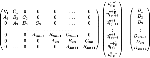
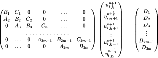
As an example, the tridiagonal system to be solved looks like (4.27) for the case when East and West sides have both level boundary-condition.

$$\begin{pmatrix}B_1&C_1&0&0&0&\dots&0\\ A_2&B_2&C_2&0&0&\dots&... ... D_3 \\ \vdots\\ D_{2m-1}\\ D_{2m}\\ D_{2m+1} \end{pmatrix}$$ (7.24)

The tridiagonal system to solve is (4.28), for the case when East and West borders sides have both flow boundary-condition.

$$\begin{pmatrix}B_2&C_2&0&\dots&0\\ A_3&B_3&C_3&\dots&0\\ \hdo... ...pmatrix}D_2\\ D_3 \\ \vdots\\ D_{2m-1}\\ D_{2m} \end{pmatrix}$$ (7.25)

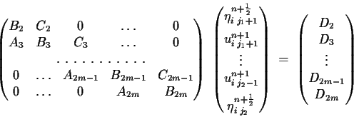
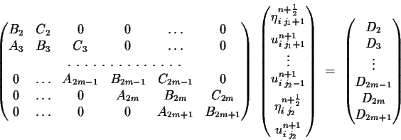
What follows are the matrix layouts for the others two possible BC: level-flow (4.29) and flow-level (4.30).

$$\begin{pmatrix}B_1&C_1&0&0&\dots&0\\ A_2&B_2&C_2&0&\dots&0\\ ... ...ix}D_1\\ D_2\\ D_3 \\ \vdots\\ D_{2m-1}\\ D_{2m} \end{pmatrix}$$ (7.26)

$$\begin{pmatrix} B_2&C_2&0&0&\dots&0\\ A_3&B_3&C_3&0&\dots&... ...\\ D_3 \\ \vdots\\ D_{2m-1}\\ D_{2m}\\ D_{2m+1} \end{pmatrix}$$ (7.27)