As far as the second-order moments of the random function ![]() are concerned, these
nested structures can be conveniently represented as the sum of a number
of variograms (or covariances), each one characterizing the variability at a
particular scale.
are concerned, these
nested structures can be conveniently represented as the sum of a number
of variograms (or covariances), each one characterizing the variability at a
particular scale.
For example,
![]() may be a transition model (spherical or exponential)
which very rapidly reaches its sill value
may be a transition model (spherical or exponential)
which very rapidly reaches its sill value ![]() for distances
for distances ![]() that are only
slightly larger than the data support. This model thus combines all the
micro-variabilities (e.g., measurement errors and petrographic differentiations).
that are only
slightly larger than the data support. This model thus combines all the
micro-variabilities (e.g., measurement errors and petrographic differentiations).
![]() may be another transition model with a larger range (e.g.,
may be another transition model with a larger range (e.g.,
![]() ) characterizing the lenticular beds and
) characterizing the lenticular beds and
![]() may be a third transition model with a range (
may be a third transition model with a range (![]() )
representing the alternation of
strata or the extent of homogeneous mineralized zones.
)
representing the alternation of
strata or the extent of homogeneous mineralized zones.
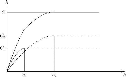
At smaller distances (![]() ), the observed total variability depends
on
), the observed total variability depends
on
![]() , cf. Figure 4.1,
while for large distances it will depend on all the
, cf. Figure 4.1,
while for large distances it will depend on all the
![]() .
.