LOW CARBON STEEL CORROSION DAMAGE PREDICTION IN RURAL
AND URBAN ENVIRONMENTS
Díaz Verónica, López Carlos, Rivero Susana
Facultad de Ingeniería-Universidad de la República Oriental del Uruguay
Abstract
This paper presents an Artificial Neural Network (ANN) model for the damage function of carbon steel, expressed in m m of corrosion penetration as a function of environmental variables. Working in the context of the Iberoamerican Atmospheric Corrosion Map Project, the experimental data comes as result of the corrosion of low alloy steel subtracts in three test sites in Uruguay, South America. In addition, we included experimental values obtained from short time kinetics studies, corresponding to special series from one of the sites. The ANN numerical model shows attractive results regarding goodness of fit and residual distributions. It achieves a RMSE value of 0.5m m while a classical regression model lies in the range of 4.1m m. Furthermore, a properly adjusted ANN model can be useful in the prediction of corrosion damage under different climatological and pollution conditions, while linear models cannot.
Keywords: atmospheric corrosion, damage function, neural networks,
pollution, rural and urban environments
Introduction
Uruguay takes part of the collaborative project MICAT (1), operating
four atmospheric corrosiveness stations. Standardized metallic samples
are exposed in different natural environments, using also standardized
procedures and environmental data collection agreed by the MICAT working
group.. Amongst meteorological ones we include hourly values of relative
humidity, temperature, wind speed and direction, as well as daily precipitation
and precipitation run in number of days. Pollution data includes monthly
values of sulfur dioxide and chloride deposition rates.
There is a significant research body regarding analytical expressions
or models (2,3,4,5,6). The economical and technological importance is fairly
clear, because meteorological and even pollution records are taken routinely,
while the corrosion rate of low alloy steel require mid-to-long term experiments.
The task has shown to be difficult, because of non-linearitys associated
with the physicochemical process responsible for the atmospheric corrosion
phenomena.
Most of the predictive models used to date are linear regression models
that fit the data such that the root mean square error is minimized. Nevertheless,
they have been shown to be effective only in few areas. Artificial Neural
Network Modeling emerges as a promising tool in corrosion research, because
of it potential to model complex non linear processes provided its architecture
and parameters are properly set.
This paper tackles the modeling of corrosion penetration in terms of
standard meteorological variables for low carbon steel alloy. We have selected
as pertinent meteorological parameters the cumulated time of wetness (in
hours), cumulated chloride deposition (in mg Cl/m2), cumulated
sulfate deposition (in mg SO2/m2), cumulated hours
with relative humidity below 40%(in hours), cumulated precipitation (in
mm), as well as mean relative humidity (in %), and mean temperature (in
°K).
The problem under investigation is one of function estimation. Given
a set of n observations at time i
of m meteorological variables Xiand
the corresponding observed corrosion penetration values fi,
i
=1...n, find f(X,P) (boldface denotes a vector) such that the mean
sum of the squared errors MSSE, defined as:

Materials
Low alloy steel subtracts, with known chemical composition (C 0.05 %, Mn 0.37 %, S 0.011 %, P 0.01 %, Cr 0.012 %, Ni 0.012%, Cu 0.021%, Ti 0.02%, As 0.01%), prepared according to ISO 8407 Standard (7), were exposed to atmospheric corrosiveness stations, covering very pure rural to industrial-urban polluted atmospheric environments. The experimental design comprised long and short term exposure series. Concerning long- term exposure periods, all the test sites have had the following exposure schedule: 3 series with one-year exposure, and one serie with two, three and four years exposure periods, respectively. Concerning short-term, an experiment was designed including five sequences corresponding to: 1, 2, 3, 5 and 7 months of exposure periods for samples located at a continental industrial- urban test site named Prado. Four specimens of each serie were exposed in each sequence, three of which were used to evaluate annual corrosion rate. The specimens were exposed in each test sites corresponding the geographical co-ordinates and major climatological parameters described in Table I.
Table I Some climatological parameters and geographical coordinates for the measuring stations
|
|
|
||
|
|
|
|
|
|
|
|
|
|
|
|
|
|
|
|
|
|
|
|
|
|
|
|
|
|
|
|
|
|
|
|
|
|
|
|
|
|
|
|
|
|
|
|
|
|
|
|
|
|
1: mean coldest month temperature, 2: mean hottest month temperature, 3: mean annual temperature, 4: minimum monthly rain, 5: maximal monthly rain, 6: mean annual rain. 7:ASL: Above Sea Level. All stations are located in areas classified as Humid Template Without Dry Season, according to Köppen scale.
Brief Introduction to Artificial Neural Networks
The term "artificial neural network" (ANN) denotes a computational structure
intended to model the properties and behavior of the brain structures,
particular self-adaptation, learning and parallel processing. It consists
of a set of nodes and a set of interconnections between them (10),(11).
A node contains a computational element (neuron) which takes inputs through
synaptic connections from some other neurons and produces a single output.
A typical neuron takes as input the weighted sum of the input links and
produces a single output through a given transfer function. The behavior
and properties of such a net is dependent of the computational elements,
in particular the weights and the transfer function, as well as the net
topology. Usually the net topology and the transfer function are specified
in advance and are kept fixed, so only the weights of the synaptic connections,
and the number of neurons in the hidden layer need to be estimated. The
usual procedure is to divide the available dataset in two parts: the learning
(or training) set and the test set. The former is presented
to the ANN, and the Mean Sum of Squared Errors MSSE(P) is minimized
by properly choosing of P. This process is denoted as training.
Once P is estimated, a verification takes place analyzing the generalization
ability of the ANN, evaluating the MSSE using the test set. Usually,
this new value is larger than the one obtained for the training set; if
they are similar or even smaller, the parameters are accepted and the ANN
is ready to be used. Otherwise, some adjustment should be made, and the
overall training process is repeated. Notice that the parameters are held
constant while evaluating the MSSE with the test set.
The transfer functions can be linear or not. The latter ones are more
often used because they allow the network to fit better the training set
than linear ones. Linear ANN can only map linear functions, severely limiting
the usefulness of the model for our purposes.
The neurons can be connected in many ways, and thus leading to different
architectures. The most popular option is named as Multilayer Perceptron
Structure. It consists of one input layer, where the connection with the
input data is performed. Such input is passed (lets say, from left to right)
to a hidden layer. All neurons in the first hidden layer receive
a weighted average of all inputs, but there is no connection among them.
If available, further hidden layers receive inputs from weighted averages
of the outputs of the previous layers. The final layer collects the inputs
of the last hidden one, and produced the output of the ANN. In our case,
we have just one neuron in the final layer, because we will produce just
a function value. Each hidden layer can have any number of neurons, and
each neuron can have (in first instance) a different transfer function.
The more neurons in the hidden layers, the more sophisticated cases the
network is capable of learning.
All the neurons receive as input a weighted average of the outputs
of the previous layer; we will denote the weights as wij,. Each
synaptic weight wij, is interpreted as the strength of the connection
from the jth unit to the ith unit. It is customary
to add a constant bias term is added in order to improve the training phase.
The input can be calculated as
![]()
where wij are the synaptic connection weights from neuron
j to neuron i, outputi is the output from neuron i, and
mj
is a bias for neuron j
The output of each neuron is a simple function of its net input. It
can be linear, but the most interesting case is the non-linear one. A number
of nonlinear functions have been used by researchers as transfer
or activation functions, for example:
![]() (Also denoted as the sigmoid
function)
(Also denoted as the sigmoid
function)
![]()
![]()
![]()
Cybenko (8) demonstrated that under weak requirements on the transfer function, an ANN with one hidden layer and enough neurons can approximate any continuous function to an arbitrary degree. The synaptic weights in neural networks are conceptually similar to coefficients in regression models. They are adjusted to solve the problem presented to the network.
Learning or training is the term used here to describe the process of finding the most suitable values of these weights. There are many different algorithms for training neural networks. Backpropagation (9) is the most popular one. It modifies the weights by moving in the direction contrary to the MSSE error function gradient. The algorithm is limited by the fact that it is sensitive to the set of initial weights, and it may get trapped in local optima; it requires in addition that the transfer function should be differentiable.
ANN modeling
In order to facilitate the learning process, the input variables were
normalized to a zero mean, unitary variance equivalents. We used in the
following the same name for the input variable or its normalized version.
The output of the ANN needs not to be normalized. In other branches of
science, the P Buckingham Theorem plus the prior
knowledge of all significant variables allow a reduction in the number
of inputs to the ANN while keeping valid the resulting model. Up to now
it is impossible to take full advantage of this, since the variables that
control the corrosion process are in general not precisely known .
The dataset is rather small, so it has been artificially enlarged.
It is well known in the ANN literature that some noise in the input is
beneficial in terms of convergence, so the learning set were duplicated
using a random perturbation of at most 5%. The final training set was composed
of 51 observations, plus 51 more obtained by perturbation. The test set
have 18 records.
The number of neurons for the input and output layer are fixed by the
number of meteorological variables (five) and the number of variables to
be predicted (one). The design of the ANN will be completed once the number
of neurons in the hidden layer and the activation function is specified.
Usually the activation function has considerable less influence in the
final results (8) so the asinh function has been selected for the hidden
layer, and the linear one for the output neuron.
As a working tool it has been used the Matlab Neural Networks Toolbox
2.0, in the context of Matlab 4.2 c.
Results and Discussion
This section presents an Artificial Neural Network model for the estimation of a damage function for low carbon steel substrates as a function of some input variables. Later we will discuss the performance of the model in terms of goodness of fit, and the residual distributions for training and testing data sets will be analyzed.
The inputs variables considered are: X1 time of wetness (in hours), X2 sulfate deposition (in mg SO2/m2), X3 precipitation (in mm), X4 hours with relative humidity below 40%(in hours),X5 chloride deposition (in mg Cl/m2), all of them cumulated over the considered period. The target value is the cumulated penetration (in m m). We recall that during training, we normalized the input variables to zero mean, unit variance.
The full ANN models output can be expressed as follows
![]() ;
; ![]()
where X is the vector of input variables normalized to a zero
mean, unitary variance. The scalar output y2 should fit the
measured penetration (without normalization)
It should be pointed out that the model with two neurons in the hidden
layer shown the best fitting capabilities, exhibiting the smallest RMSE
both for learning and testing data sets. This will be presented below.
The final weights for the ANN with two neurons in the hidden layer are
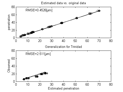
presented in figure 1. With such parameters, the RMSE for the training
set was 0.5 mm, while for the test set it was
2.5 mm which has been considered acceptable.
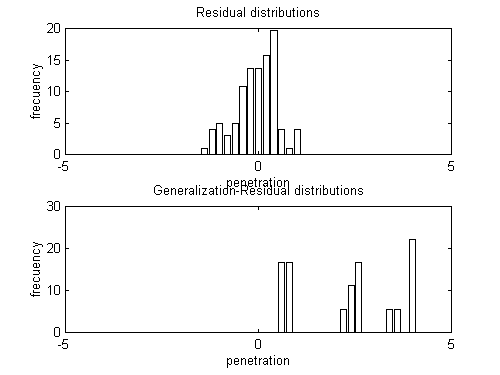
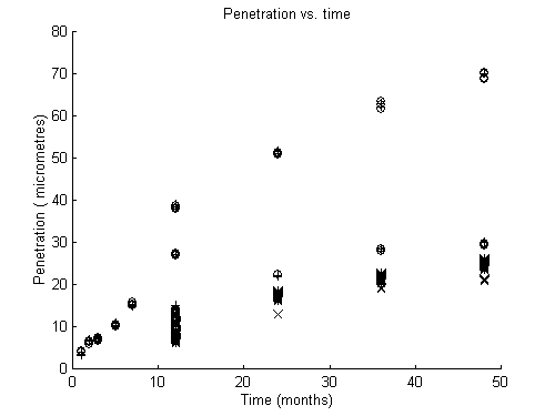
These results are graphically represented in the figure 2, additionally
with the distribution of the discrepancies between the ANN output and the
measurements as well as the evolution of the penetration in function of
the time of exposure which are respectively represented in figure 3 and
4.
|
Standard deviation = (6439 4977.4 1644.6 225.1 4779.6) Required for the normalization Mean = (7364.1 3422.5 1935.3 221.2 3171.3)
|
Figure 1. Constants for the model with two neurons and one hidden layer.
To make a comparison, we also used a classical linear regression model with the same normalized inputs. The weights were W= (-14.0104 17.0326 29.0991 7.3892 4.2913) and the constant term was 26.4930mm. In this case, the training set were fitted with an RMSE of 4.1mm, and the same figure for the test data set was 4.6mm. This show that the generalization capabilities of the linear model were good. However, the comparison with other values in the literature should be made with caution, because the researchers usually made the fit with all the available data, and reports the RMSE with such set; in that case, the ANN produces 0.5mm while the linear model 3.9mm.

Figure 2. Above, comparison of measured vs. calculated penetration
values (in mm) for the training set. Below,
the same for the testing set.

Figure 3 Distribution of the discrepancies between the ANN output
and the measurements. Above is for the training set, while below is for
the testing set.

Figure 4 Evolution of the cumulated penetration vs. time of exposure. In "o" estimated values and in "+" observed values, both for training set, in "*"estimated values , "x" observed values both for testing set
Conclusions