Towards Proactive
Network Load Management for
Distributed Parallel
Programming
Presentado en el congreso IEEE LANOMS '99 (Latin
American Network Operations and Management Symposium), (Río
de Janeiro, Brasil 1999) a cargo de S. Nesmachnow, A. López y C.
López.
Abstract
In order to increase the overall performance of distributed
parallel programs running in a network of non-dedicated workstations, we
have researched methods for improving load balancing in loosely coupled
heterogeneous distributed systems.
Current software designed to handle distributed applications
does not focus on the problem of forecasting the computers future load.
The software only dispatches the tasks assigning them either to an idle
CPU (in dedicated networks) or to the lowest loaded one (in non-dedicated
networks).
Our approach tries to improve the standard dispatching
strategies provided by both parallel languages and libraries, by implementing
new dispatching criteria. It will choose the most suitable computer after
forecasting the load of the individual machines based on current and historical
data. Existing applications could take advantage of this new service with
no extra changes but a recompilation.
A fair comparison between different dispatching algorithms
could only be done if they run over the same external network load conditions.
In order to do so, a tool to arbitrarily replicate historical observations
of load parameters while running the different strategies was developed.
In this environment, the new algorithms are being tested
and compared to verify the improvement over the dispatching strategy already
available.
The overall performance of the system was tested with
in-house developed numerical models. The project reported here is connected
with other efforts at CeCal devoted to make it easier for scientists and
developers to gain advantage of parallel computing techniques using low
cost components.
Introduction
Parallel architectures are nowadays wide spread.
With the growth of node power and the increases of network bandwidth, present
networks can be used as powerful parallel environments. This kind of hardware
support for distributed processing can be found in a growing number of
companies and universities.
However, software support for efficiently use this kind
of architectures is still not good enough. There is almost no visual environment
for developing distributed systems, and the ones that exist are extremely
expensive. On the other hand, they are (in many senses) under-developed.
In addition, they only have rudimentary tools to cope with unexpected overload
in a node. This usually leads to a significant delay in the computation
time.
CeCal [1] is concerned about this topic, and has many
concluded ([2][3][4][5]) and ongoing ([6][7][8]) research projects.
This project proposes to improve PVM [9] dispatching algorithms
in order to use historical information about the use of the computers that
compose the virtual machine. New algorithms based in neural networks techniques
and traditional statistical methods (ARMA, ARIMA) were used to predict
future usage of individual workstations based on historical usage. In order
to compare two forecasting algorithms under the same workload environment,
two instances of the same program with just the dispatching criteria changed
should be run. However, this executions should run in a background load
environment as similar as possible.
This paper describes the work done on this direction,
both about the development of new dispatching algorithms and in the infrastructure
needed to fairly compare them against the standard ones (network load gatherer
and replicator).
These new dispatching algorithms were tested using UCLA´s
Global Climate Model [10] and a Shallow Water Model. [11]
Load Balancing and new dispatching criteria
It has been proved that load balancing can be considered
as the most relevant performance enhancement in a multi-user network environment.
When many tasks are used for solving some problem, a single delay produces
the whole system be delayed, with the other tasks waiting for the delayed
one at synchronizing points. Load balancing techniques allow distributed
applications to take care about this problem.
Standard load balancing strategies for distributed applications
propose choosing the most appropriate workstation of the virtual machine.
The most appropriate workstation means the lowest loaded machine at task
spawning time. All the history of workstations load is ignored and only
instant load is considered.
Our project proposed and implemented two original methods
for improving load balancing of distributed applications. In both cases,
load balancing will be considered before tasks are started, by forecasting
load in the target computer.
By considering statistical information, load balancing
could be improved. Our project will include services in the PVM kernel
for gathering virtual machine workstations load information, and using
it at task spawning time in order to forecast future workstation load and
correctly define the "most appropriated workstation" choice. Different
time series forecasting methods were compared; predictors were implemented
and a framework was developed in order to test and compare improved vs.
traditional dispatch.
Determination of Load Meaningful Parameters
There exists many and different workload that can be considered
for load balancing improvement: number of tasks in the run queue, size
of free available memory, 1-min load average, amount of free CPU time,
and so on. In order to improve PVM dispatching routine we have to predict,
in some way, future load of the workstations that compose the virtual machine.
This prediction will be based in some combination of the selected workload
parameter. This value is usually called the load index.
In order to compare our new dispatching strategy, we need
to run the same PVM program in the same virtual machine load environment
with both the old and the new dispatching routines. So, we must be able
to generate a workload artificially, for arbitrarily replicate historical
observations of load parameters while applying the different strategies.
The framework developed for testing and comparing different
task dispatching algorithms (the Load Replicator) will be discussed below.
We needed support for replicating, at any time, a given
network load situation. Only with this artificially generated background
workload, one could fairly compare different solutions for the dispatching
of a distributed program. The input is, for N workstations, a time series
of the load observed for some representative parameters, and the output
will be each workstation loaded with the prescribed load.
UNIX systems provide at many levels of detail information
about system usage [12]. The load information we used is the one provided
by the rstat service, which gathers information about CPU usage, local
(non NFS) disk usage, paging and swapping, interrupts and context switches,
network usage and collisions. Some of them are graphically represented
in figure 1.
Looking for simplicity and transparent processing, we
discarded some parameters that have no effect in global load patterns.
For example, kernel operations like context switching were ignored because
they are extremely hard to trace and replicate, and they do not affect
global workstation performance [13]. Also, parameters related with misconfiguration
problems (for example, if excessive swapping and paging is observed, possible
exists a memory leak problem) were ignored. On the other hand, parameters
that hardly change or are not meaningful over the time (like collisions)
also were neglected.
The identification of suitable load indexes is not a new
problem [14], and is well known that simple load indexes are particularly
effective. Kunz [15] found that the most effective of the indexes we have
mentioned above is the CPU queue length. However, due to the specific topic
we are managing (network parallel computing) where network traffic is a
bottleneck and distributed processes usually make great use of local disk,
we considered that this two indexes should not be neglected.

Figure 1
Artificial Replication of Network Load Environment
Under the assumptions described, we have replicated just
CPU, disk and network usage for each workstation.
Replication is not a new research area, and it is needed
for testing purposes in many computer science areas. Workload replicators
for measuring performance of different file system implementations were
studied in [16][17]. Also replicators for real-time system applications
were developed that work at the kernel level, obtaining excellent results
for very short periods of time [14].
As our purpose is to replicate workloads in a complete
network with many parameters of each workstation, we dont need excessive
precision in the replication at the microsecond scale, but we expect acceptable
results for the long periods (like hours). So we decided to work at the
process level.
In this paper we will focus only on CPU replication; the
other parameter replication are exactly the same, just changing the loader
subprocess. The procedure is very simple: if historical load is bigger
than actual load, then we do hard work in non-cacheable tasks; if not,
we just wait. Periodically we compare both loads and we act in consequence.
Figure 2 Historical CPU load Figure
3 Replicated CPU
Despite its simplicity, this strategy works fine. We can
visually compare the historical load (figure 2) and the replicated one
(figure 3). Vertical axis shows the percent of CPU used during the measured
interval, with increments in the range 1-100 per second. Horizontal axis
indicates historical measurements, taken every 60 seconds in these experiments.
These units are used in all experiments shown in this paper, unless is
specified.
Errors obtained for CPU replication are shown in figure
4. Working with a 60 seconds interval, average deviation was of 0,97 while
the maximum deviation was 5. The vertical axis units are those provided
by rstat.
In order to measure the overhead generated by the replication
processes, producer and replicator processes could be run using zero historical
data. Also, load overhead generated by the collector process was considered.
Figure 5 shows generated load for both auxiliary processes involved in
load replication. Load overhead observed was of 0.1 % of CPU used per second,
so it could be neglected, and ensures that previous results were fairly
good for our purposes.
Disk and network replication designs were similar, although
results were not so good. Disk simulation was implemented writing random
data directly to the raw device (in order to avoid system caches). However,
some historical high data was impossible to replicate, especially when
was generated due to access to very slow devices (like CD-RROM units).
Network usage replication was rather good: the average absolute deviation
for each interval was of 25 packets/sec.
Additional information about this sub-project (and some
other related projects) could be found at [5].
Analyzing CPU usage as a representative execution time factor
In order to verify the relationship between CPU usage
and the execution time for an almost-deterministic task, a statistical
experiment was designed. It proposes to charge a specifically host and
determining the way a large system CPU usage produces an individual task
to be delayed.
Figure 4 Average deviation in CPU load replication, per second
Figure 5: generated load for both auxiliary
processes involved in load replication.
The individual task was composed with standard parallel
designed program instructions and its almost-deterministic behaviour was
tested by running it several times over a dedicated network (null network
load was present). The results are resumed and commented below.
a) Almost-deterministic behaviour over null network load
Running the test program over null network load conditions,
we determined that the execution time does not change substantially. We
also tested the behaviour of our program test running over the different
architectures that compose our parallel machine. We found very small differences
between the results, and we concluded that the test program has an almost-deterministic
behaviour. An example test result is offered in figure 6, with data collected
from machine maserati.fing.edu.uy
Figure 6: almost-deterministic test program behaviour
The average time execution was 759.75 sec. The standard
deviation of time execution was 30.92 sec., representing a 4,07% over average
time execution.
b) Relationship between CPU usage and execution time over external
load conditions
Running the test program over different load conditions
in different hosts, we confirm a pseudo-linear functional relationship
between external CPU usage and execution time. The test program was delayed
when running over a high loaded machine, and the delay seems to be a linear
function for non extreme load values. Figure 7 resumes the results obtained,
with data from volvo.fing.edu.uy
Figure 7: almost-linear relationship between external
CPU
usage and execution time
This results offer two main conclusions to bear in mind
:
1) To determine whether a dispatch strategy is better
than another one, the system performance (simply measured by the average
execution time) should be incremented in a factor over the 4% given by
the pseudo-deterministic behaviour when using the new criteria.
2) A pseudo-linear functional relationship between execution
time and external CPU usage was confirmed. As a consequence, CPU usage
reveals itself as a meaningful parameter for load balancing improvement.
So, we have to predict CPU usage in our improved load management dispatch
algorithm.
Time Series Forecasting Load Parameters
We used time series to predict load just one time step
ahead in time, using available information up to (and including) spawning
time. The implemented methods can be divided into two categories: linear
and non-linear. In the first case the estimated quantity is a linear combination
of the available data. Its general expression is  ,
being yj the unknown quantity, x a vector which entries are the available
data and b a scalar constant; both the weight vector w and the number b
depends on the method. Typically the vector x holds the values of the same
instant, and both w and b are constants.
,
being yj the unknown quantity, x a vector which entries are the available
data and b a scalar constant; both the weight vector w and the number b
depends on the method. Typically the vector x holds the values of the same
instant, and both w and b are constants.
For non-linear methods the value is assigned using a non-linear
formula. We compared a number of different methods, and due to space constraints
we will summarize those who proved successful.
The Naive prediction and the Perfect prediction were used
as reference predictors. Naive strategy is the standard PVM dispatching
rule (it assumes that load will not vary as time goes by and uses the instant
value as prediction), while the Perfect prediction is defined only in our
test environment and it consists in the best prediction method. We used
the real next value as a prediction, so the dispatch strategy could not
be improved. The idea behind this approach is to compare our new dispatching
criteria not only versus the standard methods but against the ideal one
also, in order to determine the improving accurately.
Computer load might have peak values that might be unreasonable
or unusual. In the statistical literature such values are denoted as outliers.
They can be defined as values that do not follow the pattern of the majority
of the data and thus they might affect adversely the performance of the
methods.
Linear deterministic methods
Due to their simplicity, these methods are widely used.
We worked with the Ordinary Least Squares (OLS) method; a brief description
follows: OLS is a standard method and the theory for it can be found at
[18]. The weights w are chosen in order to minimize the 2-norm of the vector
M(j)w - m(j) (a scalar proportional to the Root Mean
Square of the Errors, RMSE) where M(j) is the matrix of the
available data (as many rows as events, as many columns as computers) and
m(j) is a column vector with the j-th computer load values shifted
in time. The shift is required in order to use old values to predict the
new one; thus first entry of m(j) corresponds to the load at
time t2 while first row of M(j) hold values of the load at time
t1. The version implemented assumes that the data is outlier free, so w
can be derived from (dropping the index j) MTMw=MTm,
b=0. Notice that this method is prone to suffer from the existence of outliers;
the solution is either to remove the outliers before the calculations or
to use an estimate more robust like the ones described below.
The Ordinary Least Squares Predictor was implemented and
included into PVM library.
Non linear methods
We used Artificial Neural Networks (ANN) methods to implement
a non-linear predictor. ANN where used to fit both a univariate or multivariate
load parameters time series using available data, in order to predict new
load values for the machines in the network. (see Warner and Misra 1996;
Stern 1996 for an ANN thorough presentation).
We have distinguished two interesting cases: a) univariate
and b) multivariate time series forecasting. In the former case, only data
for one computer is considered; in the other, data from all other computers
are considered as well. We summarize the results obtained below :
a) Univariate case
The forecasting study was done using only data from one
machine, dynsys.fing.edu.uy. The rest of the data was used when necessary.
The time series was splitted into two parts: the train-set and the test-set.
The train-set consists of the first two thirds of the database and the
rest is used to measure the quality of the prediction. RMSE is used to
quantify the quality of the prediction. The RMSE is calculated using the
test-set and the predicted data for the set. The maximum and minimum errors
were also recorded.
The first ANN tried takes into account four days to predict
the fifth. The network had an input layer of four neurones and an output
layer of a single neurone. All the transfer functions used were linear.
The topology of the first network used was:
* One input layer with four neurones
* One hidden layer with four neurones that applies a
linear transfer function
* One output layer with one output neurone that apply
a linear transfer function
All the networks were trained using the following criterion:
* 100 initial solutions were sorted
* each of them was refined -trained- 100 times
* the best solution was refined 1000 times afterwards.
Maximum and minimum values from the data set are 497.5375
and 0 respectively.
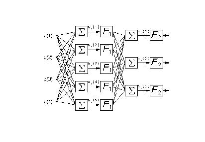
Figure 8: Sketch of a typical ANN organisation. Information flows
from left to right. There are four inputs p, one hidden layer with five
neurones with transfer function F1, a second hidden layer with three neurons
with transfer function F2 which produces three outputs. The summation symbol
indicates a weighted average of all outputs from the previous layer plus
a bias term ni(j).
The next step was to change the transfer functions used
on the hidden layers. From the results obtained we can conclude that no
significant benefits were obtained from more complex networks, at least
without further training. With this network it was possible to get a 14,5%
of benefit on the total RMS when compared with the Naive method.
All the predictions done with the borrowed network gave
a similar precision (the same order of magnitude) than the one obtained
with the locally trained network. This could be explained because all the
machines share the same profile of users, do the same kind of tasks and
have many things in common. Maybe the best predictor for a cluster of machines
like this is a common ANN trained with all the data from all the computers.
This study was not done. From the present study we can conclude that it
was not possible to make significantly better predictions with more complex
ANNs than the prediction obtained from the initial 4p1p ANN.
b) Multivariate case
We have designed and compared a number of architectures,
which vary depending on the transfer function, the number of neurones in
the hidden layer(s) and the input data. The terms purelin, logsig and tansig
and its transfer functions are defined in Demuth and Beale (1994). Despite
all of them might approximate a given function using enough neurons in
the hidden layer, we want to keep this number low for practical reasons
connected with training requirements.
The ANN named bp11 has been trained as a forecasting tool;
its inputs are the load values of the last event, and its output is the
load for the present event. It should be stressed that for each computer
a different ANN needs to be trained, using all the other load values of
the previous event as inputs. That implies 15 ANN in the CeCal net case.
All of the ANN were trained using one third of the available
records trying to minimize the RMS of the error. This approach is named
supervised learning (Warner and Misra 1996). The error is defined as the
difference between ANN output and true value. Little improvement was obtained
even under high cost (in terms of CPU) training methods were used.
Preliminary results
The integrated system was tested running a small parallel
application that simulates a parallelizable domain decomposition for a
finite difference discretization scheme. The model generates individual
tasks, dispatches them to the most suitable host; waits for the results
at a sinchronizing point, and starts over again, generating tasks using
the new values.
Preliminary results show a small improvement using average
execution time as the measurement variable over 50 samples. They are summarized
in Table 1.
|
Forecasting Method
|
Average Execution Time
|
Standard deviation
|
Improvement Over Dispatching Using Naive Prediction
|
Performance
Improvement2
|
| Naive |
796 sec.
|
17 sec. (2,13 %)
|
-
|
-
|
| OLS |
782 sec.
|
23 sec. (2,94 %)
|
14 sec. (1,79%)
|
25,9%
|
| ANN |
765 sec.
|
16 sec. (2,09 %)
|
31 sec. (4,05 %)
|
57,4%
|
| Perfect Method |
742 sec.
|
11 sec. (1,48 %)
|
54 sec. (7,27 %)
|
100%
|
Table 1 : Preliminary results.
Each sample was measured running our test program over a replicated
historical load. The test program had deterministic behaviour for every
dispatching method used. The standard deviation has always been less than
3% over average execution time.
The low improvement accomplished by the perfect method is an important
result to highlight. This method only decrease average execution time in
a 7,27% factor, even using the exact load values for the future.
Under these circumstances, the dispatching strategy based in ANN prediction
works fine, achieving half the improvement obtained by using the perfect
method.
OLS-based strategy did not work satisfactorily. It only decreases average
execution time in a 1,79% factor, which is under the limit of 2,13% given
by standard deviation of execution time.
A possible explanation for this fact is that ANN predictor can manage
load data variations in a better way than OLS predictor does. In these
cases ANN prediction outperforms the statistical methods and ANN - based
scheduler reduces the execution time.
Conclusions and further work
Load replication and new dispatching strategies have been
tested individually. Both worked satisfactorily for the purpose of this
project.
CPU load was replicated very accurately; a relative precision
of 99% was achieved when monitoring load once every minute. As our experiment
shows that for the total execution time of an application, external CPU
load was dominant over disk and network traffic, so we made not too much
effort improving disk and traffic replicators, which were not so good as
the CPU one. Further work will be done about this topic.
Several studies were made using both statistical and neural
network methods for CPU load forecasting. Load forecasting results show
that traditional statistical methods work fine and a slightly better performance
was obtained using linear ANN. We observed that more complex networks could
not improve the results obtained by simpler ones.
The primary test shows that ANN-based dispatching criteria
works satisfactorily. Dispatchers using standard statistical methods had
troubles managing load data variations.
An important preliminary conclusion is that PVM default
method is not so bad. Although we knew the load values for the future,
was not possible improve significantly the system performance, measured
in average execution time.
The next step consists in a great scale test: running
the UCLA's Global Climate and the Shallow Water Model [5] , using the new
dispatching algorithms over the same external load conditions, generated
by our replicator.
We expect to obtain good results, by decreasing the large
total execution time of this complex physical numerical model, especially
when using the ANN-based dispatch criteria. We are working in this topic
now, and results will be available in the next months.
References
-
1. Centro de Cálculo, http://www.fing.edu.uy/cecal
-
2. Estudio Comparativo de Diferentes Sistemas
Operativos para el Desarrollo de Aplicaciones Distribuidas. Alvaro Fernandez,
Pablo Prato. Technical report available at http://www.fing.edu.uy/~t5pcompa
-
3. Matlab paralelo. Pablo Stapff, Pablo Gestido.
Technical
report available at http://www.fing.edu.uy/~t5matpar
-
4. Checkpoint y Migración de Procesos
PVM en un Ambiente Distribuído. Gladys Utrera, Gustavo Atrio,Marcelo
Benzo. Technical report available at http://www.fing.edu.uy/~t5mig
-
5. Performance of a Shallow Water model and a
Global Climate Model Distributed across homogeneous and heterogeneous parallel
architectures under improved PVM dispatch. Kaplan, E.; López,
A. and López, C. http://www.fing.edu.uy/uruparallel
-
6. Modelado y Construcción de una Máquina
Paralela Virtual con Componentes de Bajo Costo. Héctor Cancela,
Ariel Sabiguero. (Instituto de Computación - Centro de Cálculo,
Facultad de Ingeniería,Universidad de la República, Uruguay).
-
7. Thesis work on PTIDAL: a Shallow Water Model
Distributed Using Domain Decomposition, Elias Kaplan,available at
http://www.fing.edu.uy/~elias.
-
8. Despacho Mejorado de Cálculo Científico
distribuido en Redes de Computadoras no Dedicadas utilizando PVM.
Carlos
López,Antonio López y Sergio Nesmachnow Centro de Cálculo,
Facultad de Ingeniería,Universidad de la República, Uruguay
-
9. PVM A Users Guide and Tutorial for Networked
Parallel Computing The MIT Press. Accesible athttp://www.netlib.org/pvm3/book/pvm-book.html10.
Wehner M. F., A. A. Mirin, P. G. Elgroth, W. P. Dannevik,C. R. Mechoso,
J. D. Farrara and. J. A.Spahr, 1995: Performance of a distributed finite
difference atmospheric general circulation model.Parallel Computing,21,
1655-1675.
-
11. Kaplan E. (1996) A shallow water model distributed
using domain decomposition. In BjorstadP., Espedal M.,and Keyes D. (eds)
Proc. Ninth Int. Conf. on Domain Decomposition Meths. (DD9).Wiley and Sons,
Bergen.
-
12. Unix System V Man pages
-
13. The Design of the Unix Operating System. Maurice
J. Bach. Prentice Hall Software series. 1986
-
14. Synthetic Workload Generation for Load-Balancing
Experiments. Pankaj Mehra, Benjamin Wah. IEEE Parallel & Distributed
Techonolgy. Vol 3. Nº3. Fall 1995.
-
15. The Influence of Different Workload Descriptions
on a Heuristic Load Balancing Scheme. T. Kunz, IEEE Trans. Software
Eng., July 1997
-
16. A User-Oriented Syntetic Workload Generator.
W-L.
Kao, R. K. Iyer. Proc. 12th Intl Conf. On Distributed Computing
Systems, CS Press, 1992, pp.270-277.
-
17. A Synthetic Workload Model for a Distributed File
Server.
R.B. Bodnarchuk, R.B. Bunt. Proc. Sigmetrics Conf. On Measurement
and Modeling of Computer Systems, ACM, 1991, pp.50-59.
-
18. Numerical Methods. Dahlquist and Bjork 1974